Building a Zipline Trading Algorithm with Custom Pipeline Factors

The Zipline python library allows us to write and test trading algorithms. We can follow the zipline tutorial to setup the library. After using the sample market data provided, or sourcing our own, running an algorithm becomes straight forward.

However, detailed information on how to build more complex and dynamic algorithms based on stock factors is not explicitly defined within the examples or documentation. Here is the example from the library that uses the Pipeline class to sort by one factor (RSI).

We will demonstrate how to filter a universe of stocks using multiple factors to create a dynamic algorithm, and use custom factors not included within the default library.

Code

Import Statements

First we will define the import statements. The order function will allow us to place orders. Next we list the imports related to pipeline that will allow us to define factor criteria. In this example we will use AnnualizedVolatility, RSI, BollingerBands as factors. We will add a custom factor later on, and we will also import pricing data to use as a criteria for stock selection.

import numpy as np
from zipline.api import order

#API imports for pipeline
from zipline.api import attach_pipeline
from zipline.api import pipeline_output
from zipline.pipeline import Pipeline
from zipline.pipeline.data import USEquityPricing
from zipline.pipeline.factors import AnnualizedVolatility, RSI, BollingerBands

Factor Instantiation

Next, all of the imported factors need to be instantiated as variables as seen on lines 5 - 9 of the snippet below. Some factors have further arguments that must be given. For example, BollingerBands compute the simple moving average of price given window_length look back periods and also the value of +/- k standard deviations from that moving average.

def initialize (context): 
    #runs once when script starts
    #context is a python dictionary that contains information on portfolio/performance.  
    #Factor criteria
    close_price = USEquityPricing.close.latest
    vol = USEquityPricing.volume.latest
    ann_std = AnnualizedVolatility(annualization_factor = 252)
    rsi = RSI(window_length = 15)
    bol252 = BollingerBands(window_length = 252, k = 2)

Custom Factor Definition

Now we will define a custom factor using the imported USEquityPricing data. A custom factor class takes as inputs an iterable of Zipline’s BoundColumn class. In this case we use USEquityPricing.close and USEquityPricing.open. We compute the average percent change over the specified window length. Note that the inputs and window length are default values and can be changed as a parameter when instantiating the custom class. The computation is actually done via numpy and should use the inputs def compute(...,close,open) passed into the compute function. Quantopian explains the basis of custom factors here. Our custom factor is computing the average price change per day over a default 10 days. Lastly we instantiate the class. The default window length is overridden. In the final code we will place the class definition before the initialize function.

class NDayMeanPctDif(CustomFactor):
    #Default inputs.
    inputs = [USEquityPricing.close, USEquityPricing.open]
    window_length = 10
    def compute(self, today, asset_ids, out, close, open):
        #Calculates the column-wise man difference, ignoring NaNs
        out[:] = np.nanmean((close - open) / open, axis = 0)

mean_pct_dif = NDayMeanPctDif(window_length = 5)

Constructing the Pipeline

Next we use the defined variables to construct a boolean expression that will constrain the factors and create a stock universe. mask_custom is the boolean expression.

1. The mask_custom boolean expression is used to set the universe of available stocks.
2. stock_basket gets the top 5 stocks with the highest average price change over the last 5 days within the mask_custom universe.

With the code below we are telling Zipline to find stocks that meet the following conditions:

1. The price is greater than $15.
2. The volume is greater than 100000 shares traded per day.
3. The price is higher than the 252 day moving average.
4. The annualized volatility of the stock is greater than 50%
5. The RSI over a 15 day period is less than 30.
6. Finally we use the custom factor to say that the average price change over a 5 day period must be greater than 1%.

    #screening
    mask_custom = ((close_price > 15) & (vol > 100000) & (close_price > bol252.middle) & (ann_std > 0.50) & (rsi < 30) & (mean_pct_dif > 0.01))
    stockBasket = mean_pct_dif.top(5, mask = mask_custom)

In the code below,pipe is the actual dataframe of the output that matches our criteria. attach_pipeline saves the pipeline settings.

    #Column construction
    pipe_columns = {"close_price": close_price, "volume": vol, 'ann_std': ann_std, 'rsi': rsi, "mean_pct_dif": mean_pct_dif}    
    pipe = Pipeline(columns = pipe_columns, screen = stockBasket)
    attach_pipeline(pipe, "Stocks")

Running the Pipeline

In Zipline the handle_data function runs every time epoch (either minute or day). The pipeline_output function gets the stocks and columns from the pipeline previously set by attach_pipeline. For this example we will buy 100 shares of each stock output by the pipeline.

def handle_data(context, data):
    context.days_stocks = pipeline_output('Stocks')
    print(context.days_stocks)

    for stock in context.days_stocks:
        order(stock, 100) 

Conclusion

We constructed a custom factor and created an algorithm that gets a dynamic universe of stocks as different stocks meet our specified requirements over time. This algorithm doesn’t complete a round-trip, but gives an idea of how to use multiple factors simultaneously. Below is the sample example code put together:

import numpy as np
from zipline.api import order

#API imports for pipeline
from zipline.api import attach_pipeline
from zipline.api import pipeline_output
from zipline.pipeline import Pipeline
from zipline.pipeline.data import USEquityPricing
from zipline.pipeline.factors import AnnualizedVolatility, RSI, BollingerBands, CustomFactor

class NDayMeanPctDif(CustomFactor):
    #Default inputs.
    inputs = [USEquityPricing.close, USEquityPricing.open]
    window_length = 10
    def compute(self, today, asset_ids, out, close, open):
        #Calculates the column-wise man difference, ignoring NaNs
        out[:] = np.nanmean((close - open) / open, axis = 0)

def initialize (context): 
    #runs once when script starts
    #context is a python dictionary that contains information on portfolio/performance.  
    #Factor criteria
    close_price = USEquityPricing.close.latest
    vol = USEquityPricing.volume.latest
    ann_std = AnnualizedVolatility(annualization_factor = 252)
    rsi = RSI(window_length = 15)
    bol252 = BollingerBands(window_length = 252, k = 2)
    mean_pct_dif = NDayMeanPctDif(window_length = 5)

    #screening
    mask_custom = ((close_price > 15) & (vol > 100000) & (close_price > bol252.middle) & (ann_std > 0.50) & (rsi < 30) & (mean_pct_dif > 0.01))
    stockBasket = mean_pct_dif.top(5, mask = mask_custom)
    
    #Column construction
    pipe_columns = {"close_price": close_price, "volume": vol, 'ann_std': ann_std, 'rsi': rsi, "mean_pct_dif": mean_pct_dif}    
    pipe = Pipeline(columns = pipe_columns, screen = stockBasket)
    attach_pipeline(pipe, "Stocks")

def handle_data(context, data):
    context.days_stocks = pipeline_output('Stocks')
    print(context.days_stocks)

    for stock in context.days_stocks.index:
        order(stock, 100)

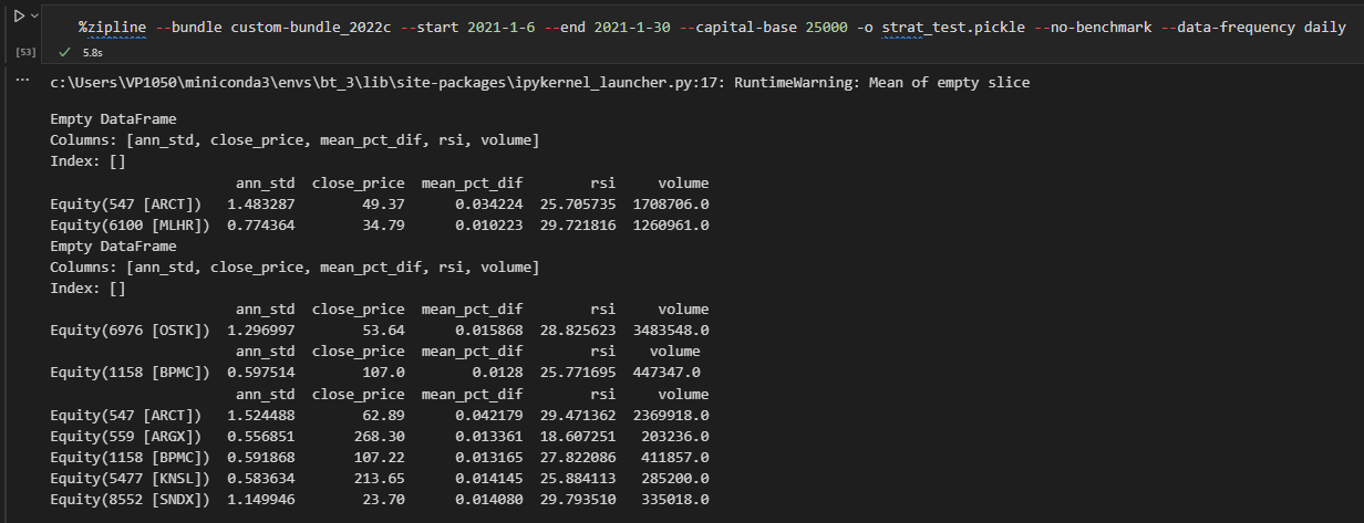
We run the code in a jupyter notebook or command line with the something like the following:

%zipline --bundle <bundle_name> --start 2021-1-6 --end 2022-2-1 --capital-base 25000 -o strat_test.pickle --no-benchmark --data-frequency daily